Imagine a straight line. Not a line segment, an infinite line. Now, imagine that line curling up so infinitely tightly that it completely fills an area, like a square, with no crossings or overlapping. How is it possible? Can a one-dimensional line fill a two-dimensional area? If so, how does it twist and turn? These questions can be answered with space-filling curves.
A space-filling curve is, as its name suggests, a line (or curve, because it is not straight) that fills a section of higher-dimensional space, such as a two-dimensional area. The most famous example is the Hilbert curve, discovered by David Hilbert.
The 0-th iteration of the Hilbert curve is a point, and each successive iteration is made by connecting four copies of the previous iteration. The Processing program below renders this curve, made from the pseudocode on this website. Use the left and right arrow keys to change the number of iterations. The diagonal line at the top-left corner is not part of the Hilbert curve, but a by-product of the algorithm used.
| hilbert_curve.pde |
Important note: None of the images in the Processing program are true Hilbert curves. The true Hilbert curve has an infinite number of iterations. As the number of iterations of a "pseudo-Hilbert curve" approaches infinity, the curve approaches a true Hilbert curve. This is true for all space-filling curves.
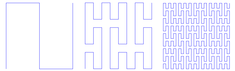
The principle of the Hilbert curve is: "Take a curve that partially fills a square and tile copies of it so that it fills a bigger square, then shrink it so it remains the same size but fills more nooks and crannies than the previous iteration". Other space-filling curves do something similar, such as the Peano curve, which tiles nine copies instead of four. This time, there is no Processing program, but here is an image of the first 3 iterations.
The principle of the Hilbert curve is: "Take a curve that partially fills a square and tile copies of it so that it fills a bigger square, then shrink it so it remains the same size but fills more nooks and crannies than the previous iteration". Other space-filling curves do something similar, such as the Peano curve, which tiles nine copies instead of four. This time, there is no Processing program, but here is an image of the first 3 iterations.
You may be thinking, "Why a square?" The answer is that a square can be tiled to make a replica of itself - that is, a larger square. This is to ensure that every iteration tiles the same shape. From the words "tile" and "replica" comes a word describing all shapes that have this property: Rep-tile. Here is an image containing a selection of rep-tiles.
Most space-filling curves have an analogous rep-tile, but the converse is not true; not every rep-tile can be made into a space-filling curve. Out of all of the rep-tiles in the image above, only three (that I know of) have a space-filling curve based on the tiling shown: the equilateral triangle in the top left, the isosceles right triangle near the top of the center, and the 30-60-90 triangle, or drafter's triangle, below the center of the image.
Well, technically, most of the rep-tiles can, but when I say "space-filling curve", I have two constraints that are not part of the real definition.
First, the curve cannot intersect itself. If it does, then it visits the same point twice, which is not aesthetically pleasing and inefficient when using it to, say, figure out a bus route. Space-filling curves are actually sometimes used for this purpose!
Second, it can't make instant "jumps" from one place to another. If you want the mathematical definition (without mathematical terms), it's:
If the distance between any two points on the curve (represented by how far along they are, where 0 is one endpoint and 1 is the other) is made arbitrarily close, the distance between them in terms of their coordinates must also be made arbitrarily close.
The Z-order curve, for example, does not satisfy the second requirement, as seen in the image below.
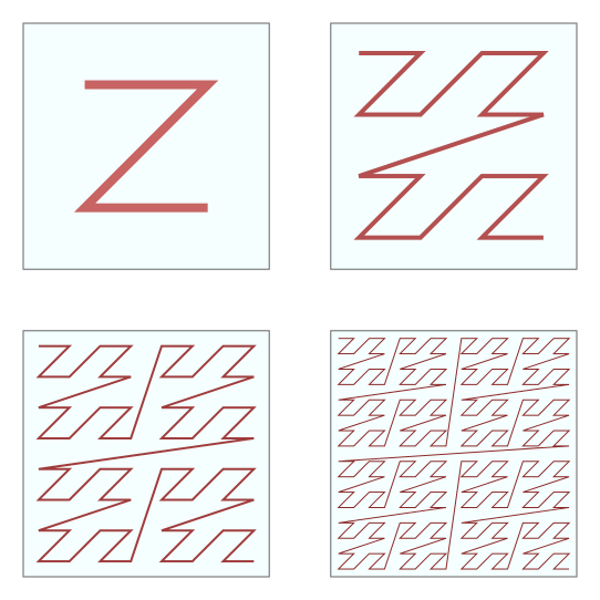
In this case, the entire curve is made of jumps, but let's focus on the biggest one, running horizontally across the center of each iteration. As the number of iterations increases, the points on either side of that jump become closer and closer in terms of percentage along the curve, as the length on either side of the jump increases exponentially. However, their distance in 2-D space never becomes shorter than the width of the square that the curve is filling.
Anyway, back to rep-tiles!
To create a space-filling curve from a rep-tile, start by subdividing it into copies of itself and connecting the centers of those copies with lines to create the first-iteration curve. Replace each subdivision with the first iteration and connect the copies to create the second iteration. Replace subdivisions with second iterations and connect them to make the third iteration. Continue as needed. Subdividing a square into four copies for this procedure creates the Hilbert curve. For the equilateral triangle, the curve would look like this:
(From 3Blue1Brown, a great YouTube channel of math videos.)
If you pause the video at a given iteration, you can see that it's made of four copies of the last iteration, arranged in the same way that an equilateral triangle's sub-copies are arranged.
For the isosceles right triangle, the corresponding curve is called the Sierpinski curve (not to be confused with Sierpinski's triangle or Sierpinski carpet, which themselves are two different things).
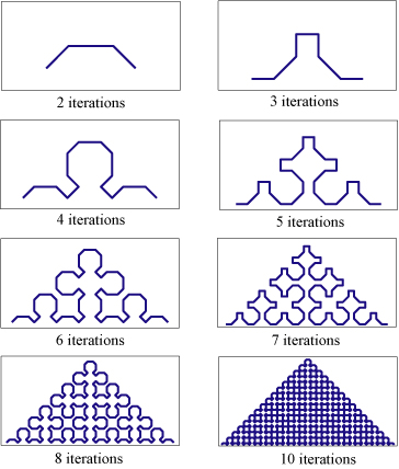
Just as the isosceles right triangle can be decomposed into two scaled-down copies of itself, this curve is made up of two of its previous iteration, connected by a line segment. However, at the level of basic shapes, it looks somewhat different than the Hilbert or Peano curves. There are squares in it, but octagons as well. Why?
It has to do with tessellations. A tessellation is a tiling, such as a grid of squares, triangles, or hexagons. For every tessellation, the centers of polygons which share an edge can be connected to form a new tessellation - its dual tessellation. For example, the dual of a triangular grid is a hexagonal one, as connecting the triangles' centers yields the hexagonal tessellation. A spacefilling curve follows the lines of the dual of the tessellation created by repeatedly subdividing its associated rep-tile.
For the Sierpinski curve, cutting the isosceles right triangle in half again and again and taking the resulting tessellation's dual gives you a grid of octagons and squares, as seen in this image from Wolfram MathWorld:
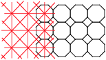
The red grid of isosceles right triangles is the result of repeatedly subdividing one triangle, and the black tessellation of squares and octagons, its dual, is the one which the space-filling curve follows.
Now we are ready to draw the curve made with the drafter's triangle. First, cut the triangle into thirds over and over, and then take its dual, which is composed of dodecagons, hexagons, and squares. Already we see that this curve will be interesting.
Now we are ready to draw the curve made with the drafter's triangle. First, cut the triangle into thirds over and over, and then take its dual, which is composed of dodecagons, hexagons, and squares. Already we see that this curve will be interesting.
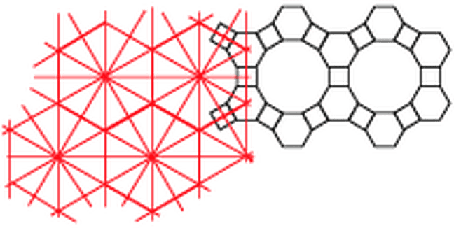
Remember, the curve will follow the lines of this tessellation of these three polygons. Start with a point as the zeroth iteration. Make three copies, arrange them like the sub-copies of the drafter's triangle, connect them with line segments, and repeat.
I originally thought that no one had created this curve before. I drew a few iterations of that curve, and then lost that drawing. Writing a Processing program to render it proved extremely difficult. I eventually found this website with an image of the drafter's curve:
I originally thought that no one had created this curve before. I drew a few iterations of that curve, and then lost that drawing. Writing a Processing program to render it proved extremely difficult. I eventually found this website with an image of the drafter's curve:
It has some very interesting features, the most obvious of which are dodecagonal "bubbles" comprising most of the curve with squares sticking out of them. In the negative space, there are hexagons. All three of these shapes are present in the dual tessellation of that of the drafter's triangle.
Space-filling curves are very strange objects, when you think about them. They are infinitely long lines that fill an area. How is that even possible? They were even considered "pathological" and "monstrous" in mathematics before the 1980's, when Benoit Mandelbrot laid the foundations for fractal geometry. These wonderfully weird objects say, "Don't always reject with what seems 'wrong'. Look a little deeper. There may be whole worlds to explore".
Space-filling curves are very strange objects, when you think about them. They are infinitely long lines that fill an area. How is that even possible? They were even considered "pathological" and "monstrous" in mathematics before the 1980's, when Benoit Mandelbrot laid the foundations for fractal geometry. These wonderfully weird objects say, "Don't always reject with what seems 'wrong'. Look a little deeper. There may be whole worlds to explore".
